
MEASURING ATMOSPHERIC ELECTRICITY
Clifford E Carnicom
Oct 21 2002
A method has been developed to measure atmospheric electrical currents and the variation of those currents within the atmosphere. Relationships between the aerosol operations and these atmospheric electrical measurements are being investigated as well. Meters that are able to measure absolute levels of current in the atmosphere appear to be difficult to acquire as well as relatively expensive. The methods described here are based upon a relatively simple electronic circuit that enjoins the use of certain mathematical procedures that hopefully compensate in part for the lack of equipment that is now available. If additional sophisticated equipment ever becomes available to meet the public needs, it will advance the process and may save considerable time and effort; approximately one a half years have been invested in the progress to date. This page will describe only the development of the method that is being used; any results from the current research will be described in a separate section. I am not an electrical technician or engineer by profession, but I have devoted considerable time and effort to the understanding of this particular circuit and JFET transistor properties. An invitation is again offered for any improvements that can be made and to review any flaws that may exist in the methods. If any errors in the method developed are identified, they hopefully can be remedied and progress can continue beyond that which has been accomplished thus far. Only fellow researchers that act in good faith on this serious topic will be engaged by this author.
This work has its origins approximately one year or more ago, when the following circuit was constructed and subsequently analyzed to begin the investigations:
BUILD THIS SIMPLE FET ELECTROMETER :
A RIDICULOUSLY SENSITIVE CHARGE DETECTOR
http://www.amasci.com/emotor/chargdet.html
This circuit was subsequently modified to the following generalized form (approximate R1 resistance value only):
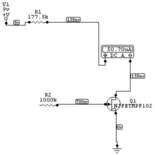
where a 50 microamp ammeter (DC A) is substituted for the earlier LED to provide some form of metric output. A variable resistor can (and has) been added into the above circuit to provided for final calibration of the meter for full scale deflection. Q1 remains as a MPF102 NJFET transistor. The application of this meter has been quite instructive and informative as to the ionic nature of our atmosphere and and the alterations that have occurred as a result of the aerosol operations. The role of positive and negative ions has also been explored in some detail, as well as the associated health effects, benefits and degradations that are ubiquitous in the literature. The initial use of this meter and certain questions that arose with its use were opened up for discussion during a previous interview with Mr. Jeff Rense (www.rense.com) on the electromagnetic aspects of the aerosol operations. At the close of that interview it was stated that the meter appeared to be recently exceeding its range of operation from unknown causes or reasons, and the exploration of the topic of atmospheric electricity was subsequently retired until my most recent re-activation of this issue a couple of months ago.
It has been surmised that the later failure of the circuit was likely due to additional experimentations involving a Van de Graaf generator, and it is suspected that the JFET transistor was damaged in the process and led to the final erroneous readings on the scale. The circuit was recently (Sept 2002) reconstructed entirely from scratch, and investigations from that point have continued from the reference levels established from earlier research.
The projected goal with the use of such a meter is to extract metric data, i.e, measurable data that can be used to to quantify both the magnitude and variation of atmospheric electrical current. Any investigations of correlation with the aerosol operations is also of value and desire. As the circuit is originally designed with the LED(light) indicator it is completely inadequate for this purpose. The meter in a light form will serve to detect the presence of positive and negative ions, but beyond that little can be accomplished. This insight into the positive and negative nature of the earth and its atmosphere is insightful and helpful to the initiate, but provides little benefit in assessing the impact of the aerosol operations.
To give the reader a sense of some of the difficulty in creating a method to measure atmospheric electrical current, the following section will be stated:
“If a needle is fastened to an insulated wire at the top of a 10 meter pole, electricity will flow from the earth to the atmosphere or vice versa. Under fair-weather skies, little if any current flow can be detected with this device since several thousand volts are required before an ordinary needle can “go into corona.“”1
Obviously it is not so simple as one might desire, and some additional methods of amplification of the signal will be needed. Hence the circuit above will at least aid in this goal, as the transistor can serve to amplify the input signal.
To give a further example of the magnitude of the problem, the fair weather current density is stated from several sources to be approximately 3E-12 amps / meter2. This means that if a square meter of conducting material was placed horizontally in the air, approximately .000000000003 amps would flow through that surface. To illustrate the problem further, if a wire (1/32inch diam., for example) was used instead of a square meter of material, the current flow would be approximately (4.95E-7meters2) *( 3E-12amps / meter2 ) = 1.5E-18 amps, or .0000000000000000015 amps. Measuring this is an impossible task at any practical level, and again the need for tremendous amplification of the signal of fair weather electricity is demonstrated. The circuit above is at least a partial step in the right direction but considerable more work is required to get any kind of measurable result.
My approach to this difficulty has been to investigate the nature of the modified circuit as it is shown and to set two conditions on the problem. They are proposed as follows:
1. The charge imparted to the electrometer (circuit) within a period of time is opposite and equal to, or opposite and proportional to the charge that is transferred from the atmosphere to the electrometer (circuit) in that same unit of time.
Notes: I have no reference for this assumption at this time; it is developed from analysis only. If we investigate the use of early electrometers by James Maxwell, however, the following descriptions of measurement of the electrical potential of the atmosphere may be relevant:
“To Measure the Potential at any Point in the Air,
Place a sphere, whose radius is small compared with the distance of electrified conductors, with its centre at the given point. Connect it by means of a fine wire with the earth, then insulate it, and carry it to an electrometer and ascertain the total charge on the sphere. ..the potential of the air at the point where the center of the sphere was placed is equal but of opposite sign to the potential of the sphere after being connected to earth, then insulated, and brought into a room.”2
The proposed assumption is in need of further examination by all researchers if an absolute magnitude is to assigned to the current measurements that result from the current research. For the sake of example to illustrate the method developed, equality of current but opposite in sign will be assumed at this time. A additional proportionality constant will remain as an unknown if this assumption is not valid. Relative current measurements and their respective variations appear to be of value at this time regardless of the outcome of this theoretical requirement that requires further validation or refutation.
For considerations on this topic as well as others in the future, the following relationships between current and voltage(potential) are provided3:
I = surface integral [ J (dot) dS ] and E = J / sigma
where I is current, J is the current density, S is a differential surface element, E is the potential and sigma is the conductivity of the material (medium).
In the case considered, J for the atmosphere can be considered as essentially constant4. This leads to I = c1 * area of conductor. Also this leads to E = c1 / sigma. Dividing both equations, we are led to ratio of I to E as: I / E = area of conductor / sigma. Since the area of the wire electrode is also a constant, we are led to I / E = c2 / sigma. The conductivity of the atmosphere does vary with altitude (increases with altitude). For the purposes and application of this research, however, it seems reasonable to regard the conductivity at ground level to remain as a relative constant also. This would lead to I / E = c2 / c3 (approx.)
or that the relationship of I to E differs only by a constant for the purposes and application of this research. This is one argument provided as to why Maxwell’s method of equality of potential is relevant to the current measurements being considered. Any comments to this subject are welcome.
2. The voltage at the gate lead of the MPF102 JFET transistor is proportional to the charge of the atmosphere. 5
Let us now formulate these premises in a mathematical form:
Qc / (t2 – t1) = – Qair / (t2 – t1)
Vg = k Qair
where Qc is the charge imparted to the circuit from the air, Qair is the charge that is transferred from the air, (t2 – t1) is the interval of time over which the measurements are taken, Vg is the gate voltage of the NJFET transistor and k is a proportionality constant.
Now the definition of current is given as6:
I = dQ /dt
where I is current, and dQ / dt is the differential change in charge with respect to a differential change in time.
Therefore,
dQ = I dt
and integrating with respect to time,
Q = integral [ I dt ]
Therefore:
Qc = integral [ Ic dt ]
where Ic is the current flowing within the electrometer circuit, integrated with respect to time.
Therefore, after multiplying each side of the equation (first assumption) by the interval (t2 – t1) and by (-1), we have:
Qair = – integral [ Ic dt ]
but from the second assumption being made, we also have:
Qair = Vg / k
Therefore:
Vg / k = – integral [ Ic dt]
or
Vg = -k * integral [ Ic dt ]
Now a model for the gate – source voltage of the MPF 102 NJFET transistor is given as7:
Id = .00063 ( Vg + 4)2 (approximation)
where Vg represents the gate – source voltage, and Id is the drain current.
Therefore,
Vg = ( Id / .00063).5 – 4
Therefore, letting Ic = Id and a = .00063,
( Ic / a).5 – 4 = -k * integral [ Ic dt ]
or
k = (- ( Ic / a ).5 – 4 ) / ( integral [ Ic dt ] )
and the proportionality constant is therefore a function of Ic, the current through the circuit.
Now from the second assumption we have:
Vg = k Qair
or
Vg = k * integral [ Iair dt ]
where Iair represents the atmospheric current flow,
and differentiating with respect to time, we have:
dVg / dt = k * Iair
or
Iair = ( 1 / k) * (dVg / dt)
To address the needs of solving for dVg /dt, current through the meter is measured over an interval of time, and a model for Vg as a function of current through the circuit has been previously given. Therefore we have:
Vg = f (Ic)
and
Ic = f (t)
Therefore, from the chain rule,
dVg / dt = ( dVg / dIc) * (dIc / dt)
now since
Vg = a-.5 * Ic.5 – b
where a = .00063 and b = 4, we have
dVg / dIc = a-.5 * (1 / 2) * Ic -.5
or
dVg / dIc = 1 / ( (2 * ( aIc ).5 )
In addition, Ic is measured with the meter over an interval of time. It has been found experimentally that Ic can be modeled both closely and realistically using a least-squares second order polynomial of the following form:
Ic = c1 * t2 + c2 * t + c3 (approximation)
where c1, c2 and c3 are coefficients of the polynomial and t is time measured in seconds. Given this form, we have:
dIc / dt = 2 * c1 * t + c2
therefore
Iair = ( 1 / k) * ( 1 / ( (2 * ( aIc ).5 ) ) * ( 2 * c1 * t + c2)
or
Iair = [ – ( integral [ Ic dt ] ) / ( ( Ic / a ).5 – 4 )] * ( 1 / ( (2 * ( aIc ).5 ) ) * ( 2 * c1 * t + c2)
and since
Ic = c1 * t2 + c2 * t + c3
we have
integral [ Ic dt ] = c1 * ( t3 / 3 ) + c2 * ( t2 / 2 ) + (c3 * t) + c0, an arbitrary constant which is equal to zero since current measurement at t = 0 is zero.
Therefore Ic in the final form for measurement is:
Iair = [ – ( c1 * ( t3 / 3 ) + c2 * ( t2 / 2 ) + (c3 * t) ) / ( ( Ic / a ).5 – 4 )] * ( 1 / ( (2 * ( aIc ).5 ) ) * ( 2 * c1 * t + c2)
where Iair is in amps.
In practice, the sequence of solving for the atmospheric current value using the electrometer is:
1. Record the times associated with current meter readings of 0, 10, 20, 30, 40 and 50 microamps respectively. It is found in practice that the total time interval for one sequence of measurements will range anywhere from several seconds to several minutes. It is found that circuit acts primarily like a capacitor in the charging characteristics and as it is expressed through current flow in the meter. It is also found that temperature has a significant effect upon the times of measurement, but does not appear to affect the outcome of the magnitude in any significant fashion. The model form as developed is reasonably complex in any attempts to characterize its behavior. It is also observed that the equation above is a function of time and the current through the meter, and it is found to reach a maximum at a reading of approximately 40 microamps at that same associated time. The interval of integration is whatever time period is required to reach a full scale deflection on the meter to 50 microamps.
2. With time vs. current readings available, solve for the least squares polynomial and coefficients as described above.
3. Evaluate the above equation as it reaches a maximum, found empirically to occur approximately at the time associated with a current reading of approximately 40 microamps.
Data that has been collected is available on the page entitled : Predicting the Operations : Sunspots and Humidity. An example of one data set and solution is available at this linked location. If proportionality is to replace equality in the first assumption being used, it is expected to make an corresponding unknown impact upon any interpretation of absolute magnitudes. The focus of the current research is upon the relative current measurements as well as variation within the process; absolute magnitude does exist as a secondary issue until methods are corroborated further. Relative measurements do appear to be of value at this time, and certain trends and patterns in the data have been identified.
This paper is provided to outline the methods which are being used to investigate this topic. Results, discussion and analysis of any findings from this research will be reported on a separate occasion. For the sake of interest, an entirely alternative method of solution has been developed using capacitance as a basis of mathematical development. The results of that alternative method appear surprisingly similar to the results of the method that has presented here. That method will not be outlined at this time unless it becomes relevant to do so. Limited time is available for my research on this as well as other topics. Professional assistance along with instrumentation is welcomed. Any comments, suggestions and recommendations may be sent to me by email at cec101@usa.com.
Clifford E Carnicom
Oct 21 2002
References:
1. Atmosphere, Vincent Schaefer, Houghton Mifflin, 1981 (inventor of cloud seeding 1941)
2. A Treatise on Electricity and Magnetism, James Clerk Maxwell, Dover, 1891
3. Electromagnetics, Joseph Edminister, McGraw Hill 1993
4. Environmental ESD, Part I : The Atmospheric Electric Circuit, by Niels Jonassen, www.ce-mag.com/archive/02/07/mrstatic.html
6. Practical Electronics for Inventors, Paul Scherz, McGraw Hill 2000, where it is stated with respect to a similarly constructed JFET electrical field meter, “The repositioning of the electrons sets up a gate voltage that is proportional to the charge placed on the object”.
7. Common Source JFET Amplifier Experiment, Bill Huffine, Dept. of Engineering Technology, University of Southern Colorado, Winter 1998 (see http://et.nmsu.edu/~etti/winter98/electronics/huffine/csamp.html).
